Learn to follow a direction.

In this notebook, we showcase the whole pipeline of

1. defining the navground scenario

2. creating the Gymnasium enviroment

3. training a policy

4. evaluating in the policy

5. saving the policy

6. using the policy in navground

in a very simple navigation task where a single agent has to move towards a target direction in an empty space, which therefore require no additional sensing information.

Steps 1 and 6 play in navground, while steps 2–5 in Gymnasium.

import warnings
warnings.filterwarnings("ignore")

Defining a scenario

from navground import sim

duration = 2.0
time_step = 0.1
scenario = sim.load_scenario("""
bounding_box:
  min_x: -1
  max_x: 3
  min_y: -1
  max_y: 1
groups:
  -
    type: thymio
    number: 1
    radius: 0.5
    control_period: 0.1
    color: blue
    kinematics:
      type: 2WDiff
      wheel_axis: 1
      max_speed: 1
    behavior:
      type: Dummy
    task:
      type: Direction
      direction: [1, 0]
    orientation:
      sampler: uniform
      from: 0
      to: 6.28
""")

In this scenario, the robot starts at a random orientation and then move rightwards. As there are no obstacles to avoid, the dummy behavior performs just fine.

from navground.sim.ui.video import display_video

world = scenario.make_world(seed=0)
display_video(world, time_step=time_step, duration=duration, display_width=300)

Creating an enviroment

import gymnasium as gym
from navground.learning import ControlActionConfig, DefaultObservationConfig
from navground.learning.rewards import EfficacyReward
import navground.learning.env

env = gym.make('navground',
    scenario=scenario,
    action=ControlActionConfig(),
    observation=DefaultObservationConfig(flat=True, include_target_direction=True),
    reward=EfficacyReward(),
    time_step=time_step,
    max_duration=duration)

The enviroment is configured to use velocity actions (linear and angular components) normalized in [-1, 1]

env.action_space

Box(-1.0, 1.0, (2,), float32)

and observations which just contains the relative target direction (as unit vector)

env.observation_space

Box(-1.0, 1.0, (2,), float32)

Training policies

Imitation Learning

We train a policy using Behavior Cloning, imitating the dummy (expert) behavior

from navground.learning.il import BC, setup_tqdm

setup_tqdm()

bc = BC(env=env, policy_kwargs={'net_arch': [8, 8]})
bc.collect_runs(1_000)
bc.learn(n_epochs=8, progress_bar=True)
bc.save("Direction/BC/model")

Reinforcement Learning

We train a policy using SAC for 20000 steps, which is the same as 1000 runs.

from stable_baselines3 import SAC

sac = SAC("MlpPolicy", env, verbose=0, policy_kwargs={'net_arch': [8, 8]})
sac.learn(total_timesteps=20_000, progress_bar=True)
sac.save("Direction/SAC/model")

Evaluating the policies

The reward is defined as min(efficacy, 1) - 1. It is zero when the agent travel at its maximal speed along the target direction. Else it is lower than zero.

The reward of an agent that does not move for the whole episode (# steps = 20) is -20.

import pandas as pd
pd.set_option("display.precision", 2)

df = pd.DataFrame()
df['still'] = {'mean': -20, 'std_dev': 0}

Let us compute the reward of the “expert” that uses the Dummy behavior.

we import evaluate_policy as

from navground.learning.evaluation import evaluate_policy

instead of

from stable_baselines3.common.evaluation import evaluate_policy

because this version supports predictor that use the info dict, which we can use to evaluate the expert.

As an alternative that rely on navground experiments, we could also run

from navground.learning.evaluation import evaluate

expert_reward_mean, expert_reward_std_dev = evaluate(env, n_eval_episodes=1_000)

from navground.learning.evaluation import evaluate_policy

reward_mean, reward_std_dev = evaluate_policy(env.unwrapped.policy, env, n_eval_episodes=1_000)
df['expert'] = {'mean': reward_mean, 'std_dev': reward_std_dev}

The policies perform similarly to the expert

from stable_baselines3.common.env_util import make_vec_env

# uses random seed
test_env = make_vec_env('navground', env_kwargs=env.spec.kwargs)

for model in (bc, sac):
    reward_mean, reward_std_dev = evaluate_policy(model.policy, test_env, n_eval_episodes=1_000)
    name = model.__class__.__name__
    df[name] = {'mean': reward_mean, 'std_dev': reward_std_dev}

df.to_csv('Direction/eval.csv')
df.T

	mean	std_dev
still	-20.00	0.00
expert	-9.01	4.49
BC	-8.18	4.46
SAC	-7.96	4.45

Displaying the policies

Let’s also check which mapping between target direction and velocity commands has been learned. Let’s start by computing the expert’s mapping:

from navground import core
import numpy as np

world = scenario.make_world()
world._prepare()
behavior = world.agents[0].behavior
angles = np.linspace(0, 2 * np.pi, 360)
dirs = np.array([core.unit(a) for a in angles])
expert_cmds = []
for angle in angles:
    behavior.orientation = -angle
    cmd = behavior.compute_cmd(0.1)
    expert_cmds.append([cmd.velocity[0], cmd.angular_speed])
expert_cmds = np.asarray(expert_cmds)

Then we can evaluate the policies

def get_cmds(model):
    cmds, _ = model.policy.predict(dirs, deterministic=True)
    cmds[:, 0] *= behavior.max_speed
    cmds[:, 1] *= behavior.max_angular_speed
    return cmds

bc_cmds = get_cmds(bc)
sac_cmds = get_cmds(sac)

and compare them

from matplotlib import pyplot as plt

fig, axs = plt.subplots(ncols=2, figsize=(12, 3))

for i, (ax, name) in enumerate(zip(axs, ('Linear', 'Angular'))):
    ax.plot(angles, expert_cmds[:, i], label="Expert")
    ax.plot(angles, bc_cmds[:, i], label="BC")
    ax.plot(angles, sac_cmds[:, i], label="SAC", alpha=0.75)
    ax.set_xlabel("angle to target direction")
    ax.set_title(f'{name} speed')

plt.legend()

<matplotlib.legend.Legend at 0x32d0c4530>

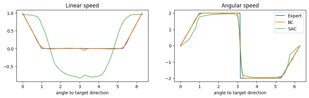
We note that the SAC policy outputs a negative linear speed, which is not feasible, according to the kinematics of the agent we selected. This happens because the outputs, before being actuated, are filtered by the kinematics, which returns the nearest feasible command.

After we compute feasible commands

kinematics = world.agents[0].kinematics

def get_feasible_cmds(model):
    cmds, _ = model.policy.predict(dirs, deterministic=True)
    twists = [kinematics.feasible(core.Twist2((cmd[0] * behavior.max_speed, 0), cmd[1] * behavior.max_angular_speed)) for cmd in cmds]
    return np.asarray([[twist.velocity[0], twist.angular_speed] for twist in twists])

bc_feasible_cmds = get_feasible_cmds(bc)
sac_feasible_cmds = get_feasible_cmds(sac)

the plots reflect better the real behavior of the agent

from matplotlib import pyplot as plt

fig, axs = plt.subplots(ncols=2, figsize=(12, 3))

for i, (ax, name) in enumerate(zip(axs, ('Linear', 'Angular'))):
    ax.plot(angles, expert_cmds[:, i], label="Expert")
    ax.plot(angles, bc_feasible_cmds[:, i], label="BC")
    ax.plot(angles, sac_feasible_cmds[:, i], label="SAC", alpha=0.75)
    ax.set_xlabel("angle to target direction")
    ax.set_title(f'{name} speed')

plt.legend()

<matplotlib.legend.Legend at 0x32d549370>

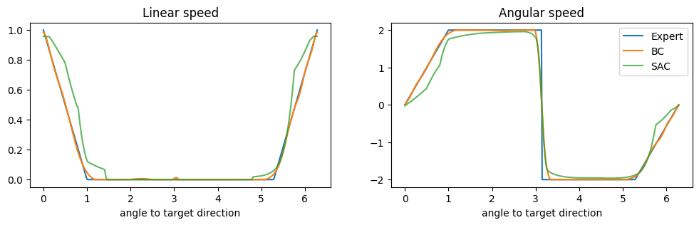
which is very similar for the three policies.

Exporting the policies

We have already saved the trained models, which we can later reload with

from navground.learning.il import BC
from stable_baselines3 import SAC

bc = BC.load("Direction/BC.zip")
sac = SAC.load("Direction/SAC.zip")

We now export to onnx, along with YAML files describing the behavior and sensor (if any) to use them.

from navground.learning import io

for model in (bc, sac):
    name = model.__class__.__name__
    io.export_policy_as_behavior(path=f'Direction/{name}', env=env, policy=model.policy)

ls Direction/BC

behavior.yaml  model.zip      policy.onnx

Using the policies in navground

For inference, we can either use the trained PyTorch policy direcly or load the onnx version

from navground.learning import onnx

policy = onnx.OnnxPolicy("Direction/SAC/policy.onnx")

They produce the same outputs

obs = env.observation_space.sample()

policy.predict(obs), bc.policy.predict(obs, deterministic=True)

((array([ 0.75968134, -0.6155738 ], dtype=float32), None),
 (array([ 0.19581495, -0.7965191 ], dtype=float32), None))

but the onnx version does it faster

%%timeit

policy.predict(obs)

5.68 μs ± 37.6 ns per loop (mean ± std. dev. of 7 runs, 100,000 loops each)

%%timeit

bc.policy.predict(obs, deterministic=True)

59.9 μs ± 695 ns per loop (mean ± std. dev. of 7 runs, 10,000 loops each)

To use them in navground, we assign a PolicyBehavior to the agent

from navground.learning.behaviors import PolicyBehavior

world = scenario.make_world(seed=0)
world.agents[0].behavior = PolicyBehavior(
    policy=onnx.OnnxPolicy("Direction/BC/policy.onnx"),
    action_config=env.unwrapped.action_config(0),
    observation_config=env.unwrapped.observation_config(0))
world.agents[0].color = 'orange'

display_video(world, time_step=time_step, duration= 2 * duration, display_width=300)

world = scenario.make_world(seed=0)
world.agents[0].behavior = PolicyBehavior(
    policy=policy,
    action_config=env.unwrapped.action_config(0),
    observation_config=env.unwrapped.observation_config(0))
world.agents[0].color = 'green'

display_video(world, time_step=time_step, duration= 2 * duration, display_width=300)

As usual in navground, we may prefer to confugure the scenario from YAML, like for the following experiment, where we alternate runs with one agent controlled by Dummy, one by the policy learned by BC and one by the policy learned by SAC.

experiment = sim.load_experiment("""
steps: 20
time_step: 0.1
record_efficacy: true
runs: 3000
scenario:
  bounding_box:
    min_x: -1
    max_x: 5
    min_y: -1
    max_y: 1
  groups:
    -
      type: thymio
      number:
        sampler: sequence
        values: [1, 0, 0]
        once: true
      radius: 0.5
      control_period: 0.1
      color: blue
      kinematics:
        type: 2WDiff
        wheel_axis: 1
        max_speed: 1
      color: blue
      behavior:
        type: Dummy
      task:
        type: Direction
        direction: [1, 0]
      orientation:
        sampler: uniform
        from: 0
        to: 6.28
    -
      type: thymio
      number:
        sampler: sequence
        values: [0, 1, 0]
        once: true
      radius: 0.5
      control_period: 0.1
      color: blue
      kinematics:
        type: 2WDiff
        wheel_axis: 1
        max_speed: 1
      color: blue
      behavior:
        type: Policy
        policy_path: Direction/BC/policy.onnx
        include_target_direction: true
        flat: true
      task:
        type: Direction
        direction: [1, 0]
      orientation:
        sampler: uniform
        from: 0
        to: 6.28
    -
      type: thymio
      number:
        sampler: sequence
        values: [0, 0, 1]
        once: true
      radius: 0.5
      control_period: 0.1
      color: blue
      kinematics:
        type: 2WDiff
        wheel_axis: 1
        max_speed: 1
      color: blue
      behavior:
        type: Policy
        policy_path: Direction/SAC/policy.onnx
        include_target_direction: true
        flat: true
      task:
        type: Direction
        direction: [1, 0]
      orientation:
        sampler: uniform
        from: 0
        to: 6.28
""")

experiment.run()

experiment.duration

datetime.timedelta(seconds=4, microseconds=105096)

efficacy = np.stack([np.mean(run.efficacy) for run in experiment.runs.values()], axis=0)

expert_efficacy = efficacy[::3]
bc_efficacy = efficacy[1::3]
sac_efficacy = efficacy[2::3]

print(f"Expert: efficacy = {expert_efficacy.mean():.2f} ± {expert_efficacy.std():.2f}")
print(f"BC: efficacy = {bc_efficacy.mean():.2f} ± {bc_efficacy.std():.2f}")
print(f"SAC: efficacy = {sac_efficacy.mean():.2f} ± {sac_efficacy.std():.2f}")

Expert: efficacy = 0.56 ± 0.22
BC: efficacy = 0.55 ± 0.22
SAC: efficacy = 0.57 ± 0.22

which, as expected, are similar to the values sampled earlier in using evalute_policy , yet now computed inside of navground.