Deadlocks and Collisions#
In this notebook, we will look at two negative events that may happen while navigating: collisions and deadlocks. We will first learn own to visualize them during a simulation, then how to perform many simulations to assess the impact of two parameters: the safety radius and barrier angle.
We are going to color colliding agents in red and deadlocked agents in blue
[1]:
from navground.sim.ui.video import display_video, display_video_from_run

def decorate(agent):
    if agent.has_been_in_collision_since(world.time - 1.0):
        return {'fill': 'red'}
    if agent.has_been_stuck_since(world.time - 1.0):
        return {'fill': 'blue'}
    return {}
We start by specifying an experiment with safety_margin=0, which is an unsafe setup that will lead to collisions.
[2]:
from navground import sim

yaml = """
type: Cross
agent_margin: 0.1
side: 4
target_margin: 0.1
tolerance: 0.5
groups:
  -
    type: thymio
    number: 20
    radius: 0.08
    control_period: 0.1
    speed_tolerance: 0.02
    kinematics:
      type: 2WDiff
      wheel_axis: 0.094
      max_speed: 0.166
    behavior:
      type: HL
      optimal_speed: 0.12
      horizon: 5.0
      tau: 0.5
      eta: 0.25
      safety_margin: 0.0
    state_estimation:
      type: Bounded
      range: 5.0
"""
[3]:
scenario = sim.load_scenario(yaml)
world = sim.World()
scenario.init_world(world, 0)
We run the simulation for some time with some agents colliding shoulder-to-shoulder.
[4]:
display_video(world, time_step=0.1, duration=120, factor=10, decorate=decorate, display_width=300)
[4]:
Try now to increase the safety margin to 0.5, which is so large that it will rapidly lead to deadlocked agents, which are colored in blue.
[5]:
yaml = """
type: Cross
agent_margin: 0.1
side: 4
target_margin: 0.1
tolerance: 0.5
groups:
  -
    type: thymio
    number: 20
    radius: 0.08
    control_period: 0.1
    speed_tolerance: 0.02
    kinematics:
      type: 2WDiff
      wheel_axis: 0.094
      max_speed: 0.166
    behavior:
      type: HL
      optimal_speed: 0.12
      horizon: 5.0
      tau: 0.5
      eta: 0.25
      safety_margin: 0.5
    state_estimation:
      type: Bounded
      range: 5.0
"""
[6]:
scenario = sim.load_scenario(yaml)
world = sim.World()
scenario.init_world(world, 0)

display_video(world, time_step=0.1, duration=120, factor=10, decorate=decorate, display_width=300)
[6]:
In between these two extrema, there should be good trade-off with no collisions and no deadlocks. We invistigate it with an experiment where we vary the safety margin.
[7]:
from navground import sim

yaml = """
steps: 3000
time_step: 0.1
record_collisions: true
record_deadlocks: true
record_safety_violation: true
record_efficacy: true
terminated_when_idle_or_stuck: true
runs: 250
run_index: 0
scenario:
  type: Cross
  agent_margin: 0.1
  side: 4
  target_margin: 0.1
  tolerance: 0.5
  groups:
    -
      type: thymio
      number: 20
      radius: 0.08
      control_period: 0.1
      speed_tolerance: 0.02
      kinematics:
        type: 2WDiff
        wheel_axis: 0.094
        max_speed: 0.166
      behavior:
        type: HL
        optimal_speed: 0.12
        horizon: 5.0
        tau: 0.5
        eta: 0.5
        safety_margin:
          sampler: uniform
          from: 0.0
          to: 0.25
          once: true
      state_estimation:
        type: Bounded
        range: 5.0
"""
[8]:
from tqdm.notebook import tqdm

experiment = sim.load_experiment(yaml)
experiment.save_directory = ""

with tqdm() as bar:
    experiment.setup_tqdm(bar)
    experiment.run(keep=True, number_of_threads=8)
We import all relevant data into a pandas frame where we also define
“safe”: no collisions
“fluid”: no deadlocks
“ok”: when safe and fluid
[9]:
import numpy as np
import pandas as pd


def count_deadlocks(deadlock_time, final_time):
    is_deadlocked = np.logical_and(deadlock_time > 0, deadlock_time < (final_time - 5.0))
    return sum(is_deadlocked)

def extract_data(experiment):
    collisions = []
    deadlocks = []
    efficacy = []
    sms = []
    bas = []
    seeds = []
    for i, run in experiment.runs.items():
        world = run.world
        sm = np.unique([agent.behavior.safety_margin for agent in world.agents])
        ba = np.unique([agent.behavior.barrier_angle for agent in world.agents])
        sms += list(sm)
        bas += list(ba)
        seeds.append(run.seed)
        final_time = run.world.time
        deadlocks.append(count_deadlocks(run.deadlocks, final_time))
        collisions.append(len(run.collisions))
        efficacy.append(run.efficacy.mean())

    df = pd.DataFrame({
        'seeds': seeds,
        'safety_margin': sms,
        'deadlocks': deadlocks,
        'collisions': collisions,
        'barrier_angle': bas,
        'efficacy': efficacy})
    df['safe'] = (df.collisions == 0).astype(int)
    df['fluid'] = (df.deadlocks == 0).astype(int)
    df['ok'] = ((df.deadlocks == 0) & (df.collisions == 0)).astype(int)
    return df
[10]:
data = extract_data(experiment)
data.describe()
[10]:
| seeds | safety_margin | deadlocks | collisions | barrier_angle | efficacy | safe | fluid | ok | |
|---|---|---|---|---|---|---|---|---|---|
| count | 250.000000 | 250.000000 | 250.000000 | 250.000000 | 250.000000 | 250.000000 | 250.000000 | 250.000000 | 250.000000 |
| mean | 124.500000 | 0.122522 | 2.236000 | 3.100000 | 1.570796 | 0.715538 | 0.856000 | 0.796000 | 0.656000 |
| std | 72.312977 | 0.072869 | 4.926396 | 12.651095 | 0.000000 | 0.125498 | 0.351794 | 0.403777 | 0.475994 |
| min | 0.000000 | 0.002141 | 0.000000 | 0.000000 | 1.570796 | 0.222478 | 0.000000 | 0.000000 | 0.000000 |
| 25% | 62.250000 | 0.055579 | 0.000000 | 0.000000 | 1.570796 | 0.700834 | 1.000000 | 1.000000 | 0.000000 |
| 50% | 124.500000 | 0.125724 | 0.000000 | 0.000000 | 1.570796 | 0.758876 | 1.000000 | 1.000000 | 1.000000 |
| 75% | 186.750000 | 0.187246 | 0.000000 | 0.000000 | 1.570796 | 0.792167 | 1.000000 | 1.000000 | 1.000000 |
| max | 249.000000 | 0.247253 | 19.000000 | 114.000000 | 1.570796 | 0.825777 | 1.000000 | 1.000000 | 1.000000 |
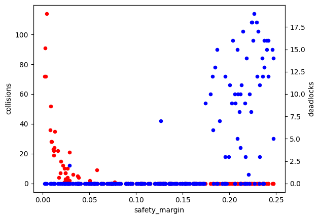
We plot the consequences of the safety margin on deadlocks and collisions. We see that
for low safety margins, there are collisions
for high safety margins, there are deadlocks
[11]:
ax = data.plot.scatter(x='safety_margin', y='collisions', color='r')
data.plot.scatter(ax=ax.twinx(), x='safety_margin', y='deadlocks', color='b');
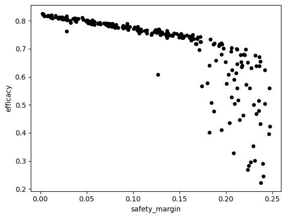
Efficacy measures how much agents are progressing towards their target (1 = ideal, 0 = stuck). Looking at efficacy gives a more fine-grained picture than deadlocks, which are still visible on the right (points lower than the slowing degrading line).
[12]:
data.plot.scatter(x='safety_margin', y='efficacy', color='k');
Deadlocks can be mitigated by reducing the barrier angle but this may cause collisions. We investigate the effect of safety margin and barrier angle with a larger experiment where we vary both parameters.
[13]:
from navground import sim

yaml = """
steps: 3000
time_step: 0.1
record_collisions: true
record_deadlocks: true
record_safety_violation: false
record_efficacy: true
terminated_when_idle_or_stuck: true
runs: 5000
scenario:
  type: Cross
  agent_margin: 0.1
  side: 4
  target_margin: 0.1
  tolerance: 0.5
  groups:
    -
      type: thymio
      number: 20
      radius: 0.08
      control_period: 0.1
      speed_tolerance: 0.02
      kinematics:
        type: 2WDiff
        wheel_axis: 0.094
        max_speed: 0.166
      behavior:
        type: HL
        optimal_speed: 0.12
        horizon: 5.0
        tau: 0.5
        eta: 0.5
        safety_margin:
          sampler: uniform
          from: 0.0
          to: 0.25
          once: true
        barrier_angle:
          sampler: uniform
          from: 0.7854
          to: 1.5708
          once: true
      state_estimation:
        type: Bounded
        range: 5.0
"""
[14]:
experiment = sim.load_experiment(yaml)

with tqdm() as bar:
    experiment.setup_tqdm(bar)
    experiment.run(keep=True, number_of_threads=8)
[15]:
data = extract_data(experiment)
data.describe()
[15]:
| seeds | safety_margin | deadlocks | collisions | barrier_angle | efficacy | safe | fluid | ok | |
|---|---|---|---|---|---|---|---|---|---|
| count | 5000.000000 | 5000.000000 | 5000.000000 | 5000.000000 | 5000.000000 | 5000.000000 | 5000.00000 | 5000.000000 | 5000.000000 |
| mean | 2499.500000 | 0.125604 | 0.501800 | 20.636600 | 1.171667 | 0.745573 | 0.59880 | 0.952000 | 0.550800 |
| std | 1443.520003 | 0.072464 | 2.484438 | 48.535728 | 0.229486 | 0.071828 | 0.49019 | 0.213788 | 0.497462 |
| min | 0.000000 | 0.000054 | 0.000000 | 0.000000 | 0.785811 | 0.208325 | 0.00000 | 0.000000 | 0.000000 |
| 25% | 1249.750000 | 0.062673 | 0.000000 | 0.000000 | 0.972600 | 0.720328 | 0.00000 | 1.000000 | 0.000000 |
| 50% | 2499.500000 | 0.127100 | 0.000000 | 0.000000 | 1.165859 | 0.760185 | 1.00000 | 1.000000 | 1.000000 |
| 75% | 3749.250000 | 0.187673 | 0.000000 | 14.000000 | 1.374103 | 0.792539 | 1.00000 | 1.000000 | 1.000000 |
| max | 4999.000000 | 0.249940 | 19.000000 | 490.000000 | 1.570597 | 0.832498 | 1.00000 | 1.000000 | 1.000000 |
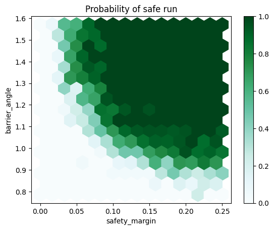
Lower barrier angles reduce safety:
[16]:
data.plot.hexbin(x="safety_margin", y="barrier_angle", C="safe",
                 reduce_C_function=np.mean, gridsize=15,
                 title="Probability of safe run");
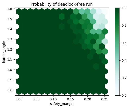
Higher barrier angles increase the probability of deadlocks:
[17]:
data.plot.hexbin(x="safety_margin", y="barrier_angle", C="fluid",
                 reduce_C_function=np.mean, gridsize=15,
                 title="Probability of deadlock-free run");
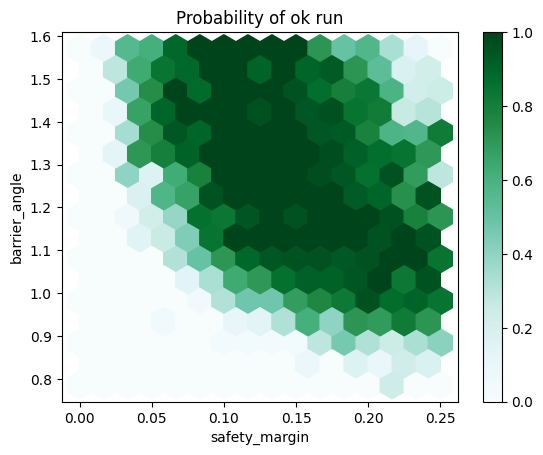
For parameters in the dark green region below, agents are behaving well:
[18]:
data.plot.hexbin(x="safety_margin", y="barrier_angle", C="ok",
                 reduce_C_function=np.mean, gridsize=15,
                 title="Probability of ok run");
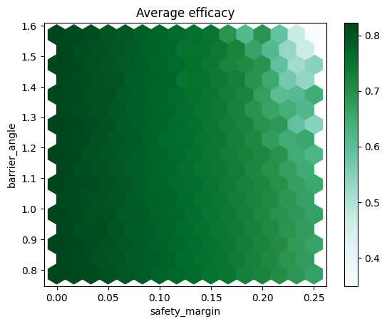
Finally, we also plot the efficacy:
[19]:
data.plot.hexbin(x="safety_margin", y="barrier_angle", C="efficacy",
                 reduce_C_function=np.mean, gridsize=15,
                 title="Average efficacy");
[ ]: