Visualize a simulation

In this tutorial you will learn how to display a simulated world as SVG or HTML in a notebook cell and how to keep the visualization synchronized.

Let’s start by definining an experiment with different types of agents

from navground import sim, core

yaml = """
type: Cross
agent_margin: 0.1
side: 4
target_margin: 0.1
tolerance: 0.5
groups:
  -
    type: thymio
    number: 10
    radius: 0.08
    color: "#e6e6e6"
    kinematics:
      type: 2WDiff
      wheel_axis: 0.094
      max_speed: 0.166
    behavior:
      type: HL
      optimal_speed: 0.12
      horizon: 5.0
      safety_margin: 0.02
      barrier_angle: 1.4
    state_estimation:
      type: Bounded
      range: 5.0
  -
    type: agent
    number: 10
    radius:
        sampler: uniform
        from: 0.05
        to: 0.2
    kinematics:
      type: Ahead
      max_speed: 0.3
      max_angular_speed: 1.0
    color: "gold"
    behavior:
      type: HL
      optimal_speed: 0.15
      horizon: 5.0
      safety_margin: 0.1
      barrier_angle: 1.4
    state_estimation:
      type: Bounded
      range: 5.0
"""
scenario = sim.load_scenario(yaml)

from which we initialize a world with a random seed:

import random

world = scenario.make_world(seed=random.randint(0, 2**31))

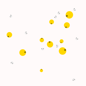
We can display the initial world state as a SVG (600 pixel width)

world

The rendering can be configured by setting world.render_kwargs like

world.render_kwargs = {'width': 300}
world

which are internally passed to the function svg_for_world which performs the rendering, and can be called direcly too:

from IPython.display import SVG
from navground.sim.ui import svg_for_world

SVG(data=svg_for_world(world, width=300))

from navground.sim.ui import render_default_config

render_default_config.width = 300
render_default_config

RenderConfig(precision=2, decorate=None, bounds=None, width=300, min_height=100, relative_margin=0.05, background_color='snow', display_shape=False, display_safety_margin=False, grid=0, grid_color='grey', grid_thickness=0.01, rotation=None, extras=[], background_extras=[])

SVG(data=svg_for_world(world))

We can embed the SVG in HTML

from IPython.display import HTML
from navground.sim.ui import html_for_world

data = html_for_world(world)
HTML(data=data)

which we can also save to a file

with open('test.html', 'w') as f:
    f.write(data)

and reload from that file

HTML(filename="test.html")

We can also render it as a png, pdf

from navground.sim.ui.render import png_for_world
from IPython.display import Image

Image(data=png_for_world(world))

or raw image.

from navground.sim.ui.render import image_for_world

image = image_for_world(world)
image.shape, image.dtype

((300, 300, 3), dtype('uint8'))

Let’s run a simulation for a while and then visualize the new world state

world.run(steps=100, time_step=0.1)

SVG(data=svg_for_world(world))

We can color the robot by their estimated time to the target.

Let’s start by defining a function that maps a value in interval [a, b] to a color, using one of matplotlib color maps

import matplotlib.colors as colors
import matplotlib.cm as cmx

def linear_map(a, b, cmap):
    c = cmx.ScalarMappable(norm=colors.Normalize(vmin=a, vmax=b), cmap=cmap)
    def f(v):
        r, g, b, _ = c.to_rgba(v)
        return f"#{int(r * 255):02x}{int(g * 255):02x}{int(b * 255):02x}"
    return f

Then we decorate the SVG fill with colors generate from the estimated times until arrival (green=almost arrived, red=still far away). Decorations are functions that map an entiry (agents, obstacles, …) to a dictionary of SVG [style] attributes.

fill_map = linear_map(0, 40.0, cmap=cmx.RdYlGn_r)

def decorate(agent):
    t = agent.behavior.estimate_time_until_target_satisfied()
    return {"fill": fill_map(t)}

SVG(data=svg_for_world(world, decorate=decorate))

We can also update the same view. For this we need to instantiate an empty canvas

from navground.sim.notebook import notebook_view

notebook_view(width=300, port=8002)

and a WebUI to keep it in sync via websockets

from navground.sim.ui import WebUI

ui = WebUI(port=8002)
await ui.prepare()

True

Let’s now populate the view withe the current simulation state

await ui.init(world)

We can change attributes on the fly. For example, let’s color all large agents in red

for a in world.agents:
    if a.radius > 0.15:
        await ui.set(a, style="fill:red")

Let’s run the simulation futher and update the view

world.run(steps=100, time_step=0.1)
await ui.update(world)

In a interative way, by iterating running and update, we could display a live simulation, which is what RealTimeSimulation does automatically for us.

from navground.sim.real_time import RealTimeSimulation

rt = RealTimeSimulation(world=world, time_step=0.1, factor=4.0, web_ui=ui)

Multiple views are supported. Let’s add one here to avoid scrolling up.

notebook_view(width=300, port=8002)

await rt.run(until=lambda: world.time > 60)

Finally, let’s color the agents by their efficacy (green=max, red=min efficacy) and run the simulation for one more minute:

fill_map = linear_map(0.0, 1.0, cmap=cmx.RdYlGn)

def f(entity):
    if isinstance(entity, sim.Agent):
        return {'fill': fill_map(entity.behavior.efficacy)}
    return {}

ui.decorate = f

await rt.run(until=lambda: world.time > 120)

We can also display a video instead of a live simulation. You need to install cairosvg (to render SVGs) and moviepy (to generate the videos)

pip install cairosvg moviepy

from navground.sim.ui.video import display_video

display_video(world, time_step=0.1, duration=30.0, factor=5.0,
              bounds=((-2.5, -2.5), (2.5, 2.5)), decorate=f, display_width=300)

or record a video to a file

from navground.sim.ui.video import record_video

record_video("test.mp4", world, time_step=0.1, duration=30.0, factor=5.0,
              bounds=((-2.5, -2.5), (2.5, 2.5)), decorate=f, width=600)

from IPython.display import Video

Video("test.mp4", width=300)

We can also first perform a run and then produce the video:

world = sim.World()
scenario.init_world(world, seed=0)
run = sim.ExperimentalRun(world, steps=500, record_config=sim.RecordConfig.all(True))
run.run()

from navground.sim.ui.video import display_video_from_run

display_video_from_run(run, factor=5.0, display_width=300)

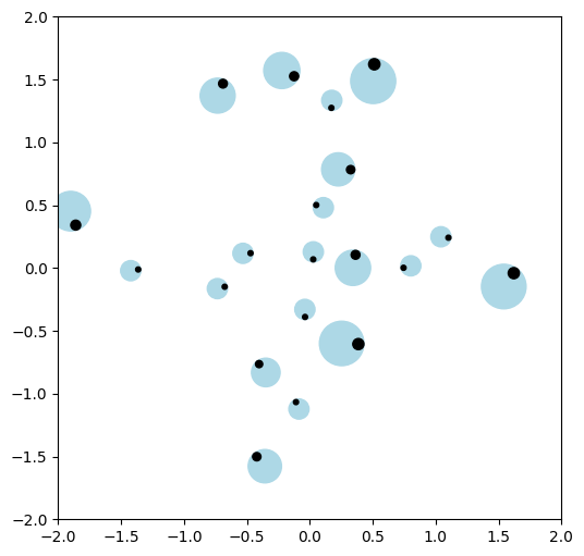
We can also use matplotlib to plot the world,

from navground.sim.pyplot_helpers import plot_world, plot_run
from matplotlib import pyplot as plt

plt.figure(figsize=(6, 6))
ax = plt.subplot()
plot_world(ax, world=world, with_agents=True, color="lightblue",
           velocity_arrow_width=0, in_box=True)

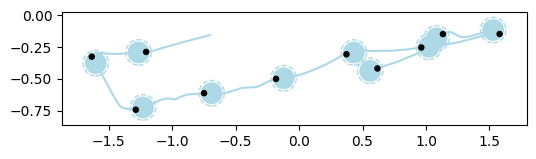
the trajectory done by one agent,

plt.figure(figsize=(6, 6))
ax = plt.subplot()
plot_run(ax, run=run, agent_indices=[0], step=50, with_agent=True,
         agent_kwargs = {'with_safety_margin': True}, color = lambda a: "lightblue")

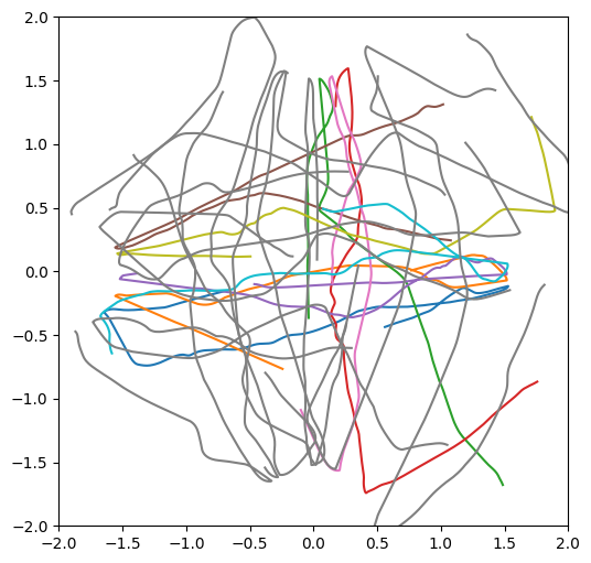
or by more agents

from navground.sim.ui import svg_color

def color(agent):
    if agent.type == 'agent':
        return 'gray'
    r = agent._uid % 10 / 10
    svg_color(r , 1 - r, 0)

plt.figure(figsize=(6, 6))
ax = plt.subplot()

plot_run(ax, run=run, with_agent=False, color=color,
         world_kwargs = {'in_box': True})