Load and playing back recorded experiments

This tutorial shows how to use the RecordedExperiment class to load, inspect and play-back a recorded experiment.

We start by recording one run of the same simple experiment as we did during the tour.

from navground import sim

yaml = """
time_step: 0.1
steps: 300
runs: 1
scenario:
    obstacles:
        - position: [5, 0.1]
          radius: 1.0
    groups:
        - number: 1
          type: thymio
          behavior:
            type: ORCA
          kinematics:
            type: 2WDiff
            wheel_axis: 2
            max_speed: 1
          task:
            type: Waypoints
            loop: true
            tolerance: 0.1
            waypoints: [[10, 0], [0, 0]]
          state_estimation:
            type: Bounded
            range: 5
          position: [0, 0]
          orientation: 0
          radius: 1.0
          control_period: 0.1
"""

experiment = sim.load_experiment(yaml)

We record all possible data

experiment.record_config.set_all(True)

to an HDF5 file, without saving the data in-memory

path = "recorded_experiment.h5"
experiment.run(keep=False, data_path=path)

We mimic closing the sessing.

del experiment

We can load the HDF5 file directly, like showcased in this tutorial, or, like we will do here, we can make use of the RecordedExperiment helper class.

We use the command line to similarly replay the record in a separate HTML view.

replay <HDF5_file>

from navground import sim
path = "recorded_experiment.h5"

recorded_experiment = sim.RecordedExperiment(path)

which exposes the a readonly version of the Experiment interface.

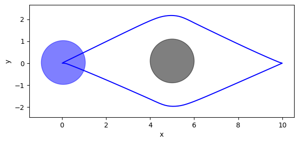
For instance, we can load the path followed by the agent

run = recorded_experiment.runs[0]
ps = run.poses
ps.shape

(300, 1, 3)

to plot it

from matplotlib import pyplot as plt

radius = run.world.agents[0].radius

fig, ax = plt.subplots(figsize=((7, 3)))
for obstacle in run.world.obstacles:
    disc = obstacle.disc
    ax.add_patch(plt.Circle(disc.position, disc.radius, color='k', alpha=0.5))
for i in range(ps.shape[1]):
    ax.plot(ps[:, i, 0], ps[:, i, 1], 'b-')
    ax.add_patch(plt.Circle(ps[-1, i], radius, color='b', alpha=0.5))
ax.set_xlabel('x')
ax.set_ylabel('y')
plt.axis('equal');

Let’s display a video of the recorded run

from navground.sim.ui.video import display_video_from_run

display_video_from_run(run)

We can also play back the recorded simulation and display it live.

from navground.sim.ui import WebUI
from navground.sim.notebook import notebook_view
from navground.sim.replay import RealTimeReplay

web_ui = WebUI(host='127.0.0.1', max_rate=-1)
await web_ui.prepare()

notebook_view(width=250)

rt_sim = RealTimeReplay(run=run, factor=5, web_ui=web_ui)
await rt_sim.run()

We can also jump to a step. Let’s go to when the agents is nearest to the obstacles:

import numpy as np

p = run.world.obstacles[0].disc.position
step = np.argmin(np.linalg.norm(ps[:, 0, :2] - p, axis=1))
run.go_to_step(step)
await rt_sim.update()

The view will then display an image similar to

from IPython.display import Image
Image(filename='playback.png', width=250)

We could also do something more interesting, like changing some parameters and executing a new simulation to compare the resulting trajectories.

For instance, let us increase the safety margin of the agent

agent = run.world.agents[0]
agent.behavior.safety_margin = 0.25

Then we perform a simulation until the end of the run, recording the new trajectory

new_ps = []

while run.world.step < run.recorded_steps:
    run.world.update(time_step=run.time_step)
    new_ps.append(np.array(agent.pose.position))

new_ps = np.asarray(new_ps)

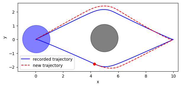
We plot in blue the original recorded trajecotory (with safery margin 0) and in red the new portion of trajecotry (with safety margin 0.25)

fig, ax = plt.subplots(figsize=((7, 3)))
for obstacle in run.world.obstacles:
    disc = obstacle.disc
    ax.add_patch(plt.Circle(disc.position, disc.radius, color='k', alpha=0.5))
ax.plot(ps[:, 0, 0], ps[:, 0, 1], 'b-', label='recorded trajectory')
ax.plot(new_ps[:1, 0], new_ps[:1, 1], 'ro')
ax.plot(new_ps[:, 0], new_ps[:, 1], 'r--', label='new trajectory')
ax.add_patch(plt.Circle(ps[-1, i], radius, color='b', alpha=0.5))

ax.set_xlabel('x')
ax.set_ylabel('y')
ax.legend()
plt.axis('equal');